This page guides you through the process of creating a lava flow using Chaos Phoenix 5 and V-Ray 5.
Overview
This is an Advanced Level tutorial. The workflow for setting up the shot, and the Phoenix settings involved in the simulation are explained in detail. However, it's recommended that you have at least basic knowleage in lighting, materials, and the Phoenix simulation.
This tutorial shows how to create a lava flow with Phoenix. The liquid stream contains liquids with various viscosity, making black patches appearing within. Therefore, this tutorial can also be used for the iron liquid usually seen in an Iron Foundry.
We simulate two liquid sources with different viscosity at different speeds. A Particle Tuner is used for simulating the molten process of lava. With the help of Grid RGB and Grid Viscosity textures, we can create a convincing lava flow both in morphology and shading.
This simulation requires Phoenix 5 Official Release and V-Ray 5, Update 2.3 Official Release for 3ds Max 2019 at least. You can download nightlies from https://nightlies.chaos.com or get the latest official Phoenix and V-Ray from https://download.chaos.com. If you notice a major difference between the results shown here and the behavior of your setup, please reach us using the Support Form.
To download project files: Download Project Files
Want to follow along but don’t have a license?: Download Free Trial
Units Setup
Scale is crucial for the behavior of any simulation. The real-world size of the Simulator in units is important for the simulation dynamics. Large-scale simulations appear to move more slowly, while mid-to-small scale simulations have lots of vigorous movement. When you create your Simulator, you must check the Grid rollout where the real-world extents of the Simulator are shown. If the size of the Simulator in the scene cannot be changed, you can cheat the solver into working as if the scale is larger or smaller by changing the Scene Scale option in the Grid rollout.
The Phoenix solver is not affected by how you choose to view the Display Unit Scale - it is just a matter of convenience.
Go to Customize → Units Setup and set Display Unit Scale to Metric → Centimeters.
Also, set the System Units such that 1 Unit equals 1 Centimeter.

Scene Layout
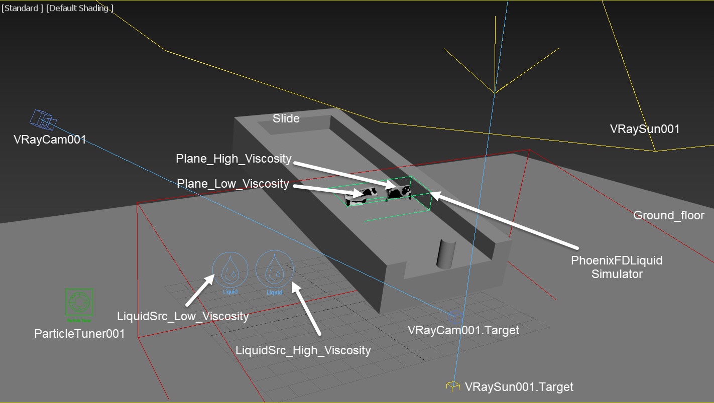
The final scene consists of the following elements:
- A Slide geometry for the lava to flow over.
- A Cylinder geometry for the flow to collide with, creating more interesting results.
- Two Phoenix Liquid Sources, one uses Plane_High_Viscosity and the other uses Plane_Low_Viscosity as Emitter Nodes.
- A Phoenix Liquid Simulator with some tweaks in the Grid, Dynamics and Rendering rollouts.
- A Particle Tuner used to tweak the Viscosity of the liquid during the simulation.
- A V-Ray Physical camera (VRayCam001) with minor tweaks for final rendering.
- A V-Ray Sun Light.
A Box geometry (Ground_floor) used as a ground.
The Plane_High_Viscosity and Plane_Low_Viscosity objects are exactly the same geometry and have the same Noise modifier applied. The only difference is their object names.
The two planes, Plane_High_Viscosity and Plane_Low_Viscosity, have Shell, Edit Poly and Noise modifiers applied.
The purpose of the Shell Modifier is to give the planes volume by turning them into an actual 3D shape with thickness. Phoenix (and fluid simulators in general) don't work well with open geometry. This ensures that the Liquid Source can properly voxelize (turn into a volume) the geometry.
The first Edit Poly modifier deletes some faces of the primitive plane.
In the second Edit Poly modifier, we select one side of the mesh, and set the face ID to 2, so we can limit the fluid emission to only one side of the mesh.
The animated Noise modifier is added to make the fluid emission more dynamic.

Here are the dimensions for the Slide geometry: 150 cm length, 60 cm width and 22 cm thickness. Angle of inclination is 13°.
The dimensions for the Cylinder geometry: 12 cm height and 3 cm in radius.

Scene Setup
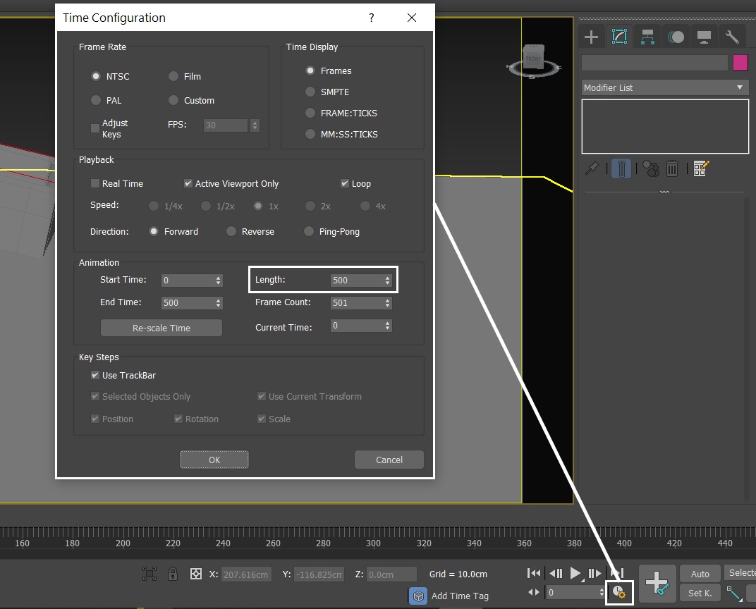
Set the Time Configuration → Animation Length to 500 so that the Time Slider goes from 0 to 500.
In this tutorial we have many steps to follow. To keep it concise, let's focus only on the Phoenix related steps and feel free to use the camera and light settings in the provided sample scene.
For your reference, below you can find the light and camera settings.
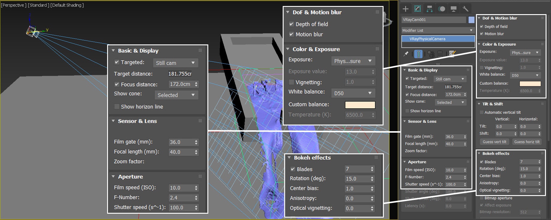
Camera Setting
Add a Command Panel → Cameras → V-Ray → VRayPhysicalCamera.
The exact position of the Camera is XYZ: [ 150.0, -156.0, 129.0 ].
The Focus Distance is set to 172.0.
The exact position of the Camera Target is XYZ: [ 101.0, -9.0, 34.0 ].
Aperture → F-Number is set to 2.4.
Aperture → Shutter Speed is set to 100.
Color & Exposure → White Balance is set to D50 with RGB color (255, 210, 160).
In the Bokeh effects tab, the Blades option is enabled and set to 7, with a Rotation of 15. Center bias is set to 1.0.
Lighting
From Command Panel → Lights → V-Ray → VRaySun, create a VRaySun in the scene.
The exact position of the VRaySun is XYZ: [ 189.5, -61.5, 190.0 ].
The exact position of the VRaySun Target is XYZ: [ 94.5, -4.0, 0.0 ].
Decrease the Intensity multiplier to 0.005.
Increase the Size multiplier to 10.0.
VRaySun acts as a directional light, yet the sun disk provides reflection source for the lava material.

Anatomy of the Lava Flow
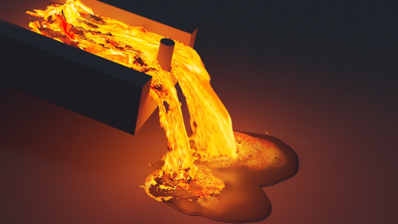
The image here is the final render in this tutorial.
Basically, we have two different types of lava in the stream. One with low viscosity, and another with high viscosity. You can see the black patches float within the hot lava due to the high viscosity liquid. When the stream flows down the slide, after it hits the ground, it starts to solidify gradually. And you can see the lava's color becomes darker as it solidified over time.
Let's go through the steps of this tutorial and see how to build these features.

Phoenix Simulation
Let's create a Liquid Simulator. Go to Modify Panel → Create → Geometry → PhoenixFD → PhoenixFDLiquid.
The exact position of the Simulator in the scene is XYZ: [ 33.4, -1.7, 58.8 ].
The exact rotation of the Simulator in the scene is XYZ: [ 0.0, 13.0, 0.0 ].
Open the Grid rollout and set the following values:
- Scene Scale: 1.0;
- Cell Size: 0.262 cm;
- Size XYZ: [ 65, 164, 33 ] - we keep the Simulator size small enough to cover only the two planes (Plane_High_Viscosity and Plane_Low_Viscosity) for liquid emission;
- Adaptive Grid: the Adaptive Grid algorithm allows the bounding box of the simulation to dynamically expand on-demand; Extra Margin to 2;
- Enable Expand and Don't Shrink;
- Enable Max Expansion: X: (28, 621), Y: (0, 0), Z: (208, 6) - to save memory and simulation time by limiting the Maximum Size of the simulation grid.
We rotate the Simulator, make it aligning (by 13°) with the Slide geometry. By doing so, we can save some simulation time.


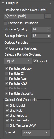
Open the Output rollout and enable the Particle Velocity, Particle RGB, Particle Viscosity, Grid Liquid, Grid RGB, Grid Velocity and Grid Viscosity Channels.
Any channel that you intend to use after the simulation is complete, needs to be cached to disk. For example:
- Velocity is required at render time for Motion Blur.
In this case, we don't enable the Particle Age channel, because we only use the Distance condition for the Particle Turner. However, if you intend to use Age as a condition, be sure to enable the Particle Age channel here.
List of Liquid Sources and their Settings
Let's create two different Liquid Sources. As an overview, we list them here first.
As the name implies, the LiquidSrc Low Viscosity emits liquid with lower viscosity, and the LiquidSrc High Viscosity emits liquid with higher viscosity.
Let's create the Sources.
We create two Liquid Sources at this step, so we can specify their Outgoing Velocity separately.
LiquidSrc Low Viscosity (Light Lava) | LiquidSrc High Viscosity (Dark Lava) | |
|---|---|---|
| Emit from | Plane_Low_Viscosity | Plane_High_Viscosity |
Outgoing Velocity | 40 cm | 20 cm |
Mask | Stucco map A | Stucco map B |
RGB | 255, 84, 0 | 0, 0, 0 |
RGB Map | Noise map (Low_Viscosity_RGB_Color) | - |
Viscosity | 0.09 | 1.0 |
Polygon ID | 2 | 2 |
Add Low Viscosity Liquid Source
Now let's add a Liquid Source from Helpers → Phoenix FD → Liquid Source. Rename the Source to LiquidSrc_Low_Viscosity.
The Liquid Source is a Phoenix helper node used to tell the Simulator which objects in the scene will emit, how strong the emission will be, etc.
Add the Plane_Low_Viscosity geometry to the Emitter Nodes list.

Once the emitter is added, set the Outgoing Velocity to 40.0cm.
Emit Mode to Surface Force.
Set the color swatch to RGB (255, 84, 0).
Set the Viscosity to 0.09.
Set the Polygon ID to 2.
At this stage, we don't map the RGB color of this Source with procedural texture, we only give it a solid color. Since this is a relatively low-resolution sim, it might downgrade the mapped Grid RGB in the shading. However, in the final simulation, when we up-res the grid, we plug a texture in the RGB slot.
The Phoenix Source in 3ds Max can use the Polygon IDs as a 'mask' - only the faces with a given ID are used for emission.
In this scene, we set the Polygon ID parameter to 2. This forces the Liquid Source to emit only from the polygons with the specified ID value.

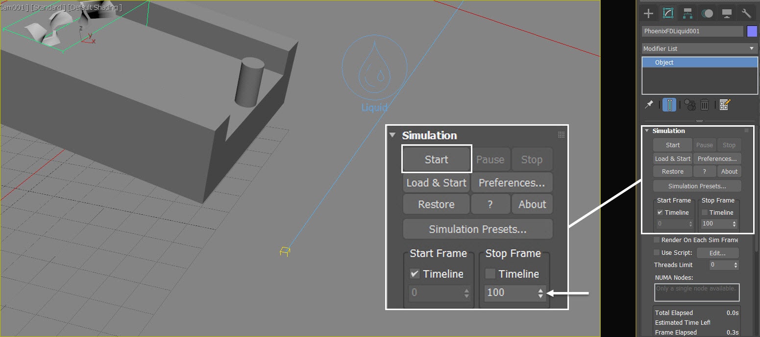
At this stage, we don't have to simulate the full length of the animation. We only need a sample, so set the Simulation rollout → Stop Frame to 100.
Press the Start button to simulate.
Go to the Preview rollout and enable Show Mesh. Disable all other Voxel Preview channels so they don't interfere.

Here is a preview animation of the simulation up to this step.
Slow Down the Liquid
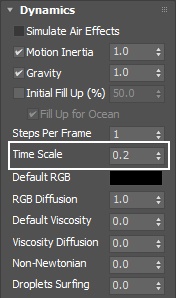
Now the liquid seems to be running too fast.
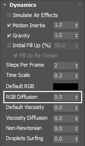
To slow it down, change the Time Scale from 1.0 to 0.2.
With the new Dynamics settings, run the simulation again.
Here is a preview of the slower simulation.
The low value of the Time Scale option smooths out the jagged look of the liquid.
Mask the Low Viscosity Liquid Source Emission
We want to emit liquid from two geometries that occupy the same space and have the same shape, but we don't want the two liquids interfering with each other. So, let's mask the emission with a Texture map. The two Stucco maps are set to complement each other. These maps can save us random flying liquids at the beginning of the emission.
Drag in the Stucco map (naming it Stucco_A) to the Texture slot next to the Mask. Make sure to choose the Instance setting (as the Copy option creates a copy of this map - you want to use the same texture for both sources instead of being forced to deal with 2 separate Stuccos).
Here are the values for the Stucco parameters:
Size: 4.0;
Thickness: 0.0;
Threshold: 0.5;
Color #1 to RGB (255, 255, 255);
Color #1 to RGB (0, 0, 0).
With the new Mask settings for the Liquid Source, run the simulation again.

Here is a preview of the simulation up to this step.
As you can see, only part of the Plane_Low_Viscosity is emitting liquid.
Add High Viscosity Liquid Source
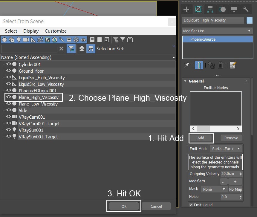
Now, add a Helpers → Phoenix FD → Liquid Source. Rename the Liquid Source to LiquidSrc_High_Viscosity.
Add the Plane_High_Viscosity geometry to the Emitter Nodes list.
Once the emitter is added, set the Outgoing Velocity to 20.0cm.
Emit Mode to Surface Force.
Set the color swatch to RGB (0, 0, 0).
Set the Viscosity to 1.0 and the Polygon ID to 2.

Mask the High Viscosity Liquid Source Emission
Drag in the Stucco map (naming it Stucco_B) to the Texture slot next to the Mask. Make sure to choose the Instance setting.
Here are the values for the Stucco Parameters rollout:
Size: 4.0;
Thickness: 0.0;
Threshold: 0.6;
Color #1 to RGB (0, 0, 0);
Color #2 to RGB (255, 255, 255).
With the new Mask settings for the Liquid Source, run the simulation again.
Note that the two Stucco maps (Stucco_A and Stucco_B) are carefully designed, so the emissions of the two Liquid Sources complement each other and are not overlapping. Specifically, the Threshold for Stucco_A is set to 0.5, while for Stucco_B is set to 0.6. Also, Color #1 and #2 in Stucco_A are opposite to the settings for Stucco_B. Make sure to set them correctly.

Here is a preview of the simulation.
With the two Liquid Sources in the scene, now the flow becomes more interesting. However, with the Mesh Preview, we can not tell which is the thick viscous liquid and which the thin liquid.
If you get some random flying particles in your liquid simulation, the reason might be incorrectly set masking texture (the Stucco map), causing the two liquids "fighting" each other.
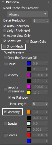
To get a viewport preview of the Viscosity channel, disable the Mesh Preview (if enabled) and enable the Viscosity channel at the bottom of the Voxel Preview section. You can also disable all other Voxel Preview channels so they don't interfere.
We need more frames for the lava flow to hit the ground.
Set the Simulation rollout → Stop Frame to 200.
Let's see a preview animation.
The thick lava now shows bright red color, while the low viscous lava shows in a darker color. Thick lava patches flow in the stream.
The default viscosity preview colors do not properly represent the actual color of a lava flow. Customization of the preview voxel color is in the later steps.
Increase Surface Tension
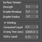
With the Simulator selected, go to the Dynamics rollout and increase the Surface Tension Strength to 0.2.
With the new Dynamics settings, run the simulation again.

Let's preview the simulation up to this step.
With the new Surface Tension setting the flow appears thicker and looks more convincing.
Enable Wetting Option
It's important to note that using Viscosity does not automatically make the liquid sticky. Stickiness can be enabled explicitly from the Wetting parameters section.
Sticky Liquid produces a connecting force between the WetMap particles at the geometry surface and nearby liquid particles.
With the Simulator selected, go to the Dynamics rollout and enable the Wetting option. Set the Sticky Liquid to 0.21.
Let's preview the simulation up to this step.
The Wetting and Sticky Liquid options further enhance the realism of the lava flow. The liquid sticks to the slide and the collider, slowing down the stream, making the lava even more convincing.
Solidify with a Particle Tuner
Next, we want to simulate the solidification process of lava. We are going to use the Particle Turner for this task.
Add a Helpers → Phoenix FD → ParticleTurner. Place it anywhere in the scene.
Click on the Edit Condition button to change condition.
The Particle Tuner assesses all particles in the simulation and changes their values if they pass a certain condition.
In this example we raise the viscosity of the particles hitting the ground.
The conditions can be very simple, but you can also build more complex conditions with the Particle Tuner's Expression operators.

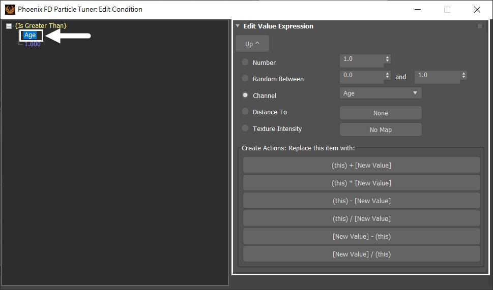
In the Edit Condition window, click on Age, then the Edit Value Expression window shows up.
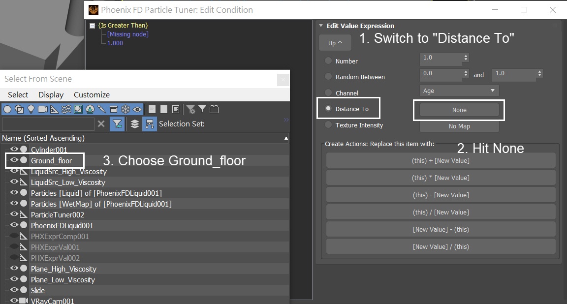
Switch the condition from Channel - Age to Distance To. Press the None button and choose the Ground_floor geometry in the scene.
Click on the 1.000 on the left.

Now you can see the Edit Value Expression window. Change the mode from Number to Random Between. Set the values to 0.0 and 30.0.
Note that the unit for distance is in simulation grid voxels. If you change the Simulator's Grid Resolution, so does the actual distance to the particle affected by the Particle Turner.

Click on the Is Greater Than, so the Edit Compare Expression window shows on the right. Change the condition from Is Greater Than to Is Less Than.
Now we have our condition set, close the Edit Condition window.

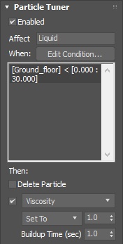
Change the affect channel to Viscosity. In the drop-down, select Set To. Make the value to 1.0. Buildup Time to 1.
Here is the final expression tree:
- If the distance to the Ground_floor is less than a Random value Between 0.0 and 30.0.
Then the Viscosity is set to 1.0.
Over the Buildup Time which is set to 1 second.
If the Buildup Time is set to 0, the specified Action is executed for every step of the simulation. If the Steps per Frame parameter of the Simulator is set to a value higher than 1, the specified Action is executed multiple times for a single frame.
Time Scale different than 1 affects the Buildup Time of the Particle Tuners. In order to get predictable results adjust the Buildup Time using this formula:
Time Scale * Time in frames / Frames per second.
Let's do a little calculation: The Buildup Time we set here is 1; Time Scale is set to 0.2; the Frame Per Second is 30; The lava flow touches the ground plane at frame 140. Therefore:
Actual Buildup Time in frame = Buildup Time / Time Scale * Frame Per Second = 1/0.2 * 30=150; 140 + 150 = 290.
So, at Frame 140, when part of the lava is less than 30 voxels distance from the ground plane, it begins to molten. At Frame 290, those particles are fully solidified, as their viscosity reaches the value of 1.0.
We need more frames for the lava flow to hit the ground.
Set the Simulation rollout → Stop Frame to 400.
With the new Particle Turner in the scene, press the Start button to simulate.

Here is a preview animation of the simulation. As you can see, the lava now solidifies as it settles on the ground.
Here is a better preview with the Viscosity channel preview on. The voxel turns red as the lava solidifies.
Increase Steps Per Frame
To make the liquid look even thicker, with the Simulator selected, go to Dynamics rollout and increase the Steps Per Frame to 2.
With the new settings, run the simulation again.

Let's see the simulation at this step.
Now, the overall look of the lava flow is taking shape. Until now, we haven't touched the shading part.
So let's first take a look at our current RGB channel data preview, since the RGB channel could be useful for shading the lava flow.
Let's make a preview of the Grid RGB channel and see what we currently have.
Select the Simulator, go to the Preview rollout. To get a viewport preview of the RGB channel, disable the Mesh Preview (if enabled) and enable the RGB channel at the bottom of the Voxel Preview section. You may also disable all other Voxel Preview channels, so they don't interfere.

As seen in the Grid RGB voxel preview, there are not many details - only black and red solid colors. Besides, the black voxels quickly blur out and we can not see any pattern in the Grid RGB.
We can easily fix the blurriness of the RGB preview issue by setting the RGB Diffusion value of the Simulator to 0.0. We see how this issue is resolved in the next run of the simulation.
Map the Grid RGB and Final Simulation
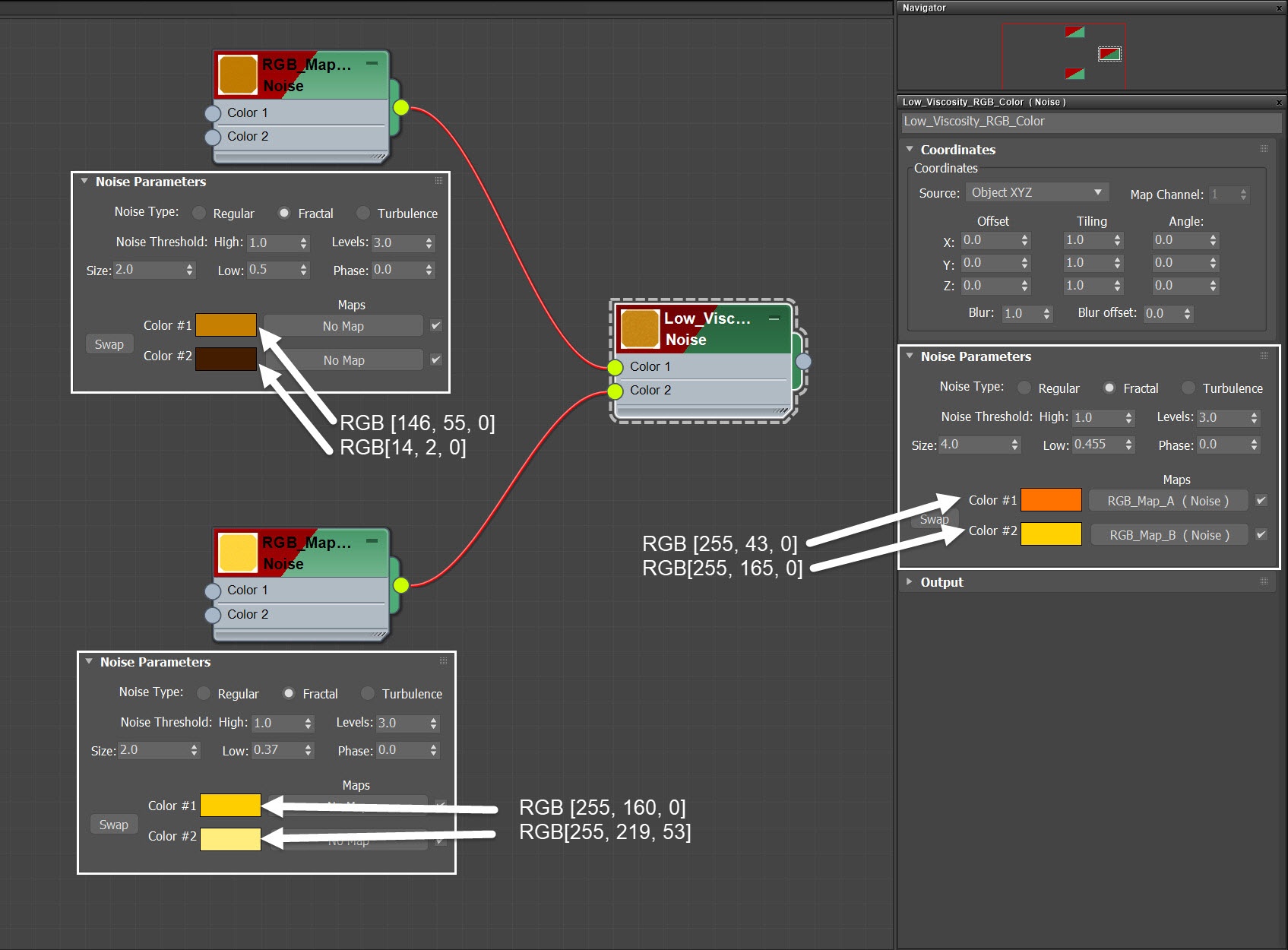
In the Material Editor, create a Noise texture and name it Low_Viscosity_RGB_Color.
Set its Size to 4.0; High to 1.0; Low to 0.455; Noise Type to Fractal.
For the Color #1 and Color #2 slots of the Low_Viscosity_RGB_Color plug another two Noise textures. Rename them to RGB_Map_A and RGB_Map_B respectively.
For the RGB_Map_A:
Set its Size to 2.0; High to 1.0; Low to 0.5; Color #1 to RGB (146, 55, 0); Color #2 to RGB (14, 2, 0); Noise Type to Fractal.
For the RGB_Map_B:
Set its Size to 2.0; High to 1.0; Low to 0.37; Color #1 to RGB (255, 160, 0); Color #2 to RGB (255, 219, 53); Noise Type to Fractal.
You don't have to set the RGB color for Color #1 and #2 of the Low_Viscosity_RGB_Color. We make them orange and yellow here just for a visual guidance. This does not affect the final shading in any way.
Once Low_Viscosity_RGB_Color is ready, drag it to the RGB slot of the LiquidSrc_Low_Viscosity Source (as an Instance).

We're all set for the final simulation.
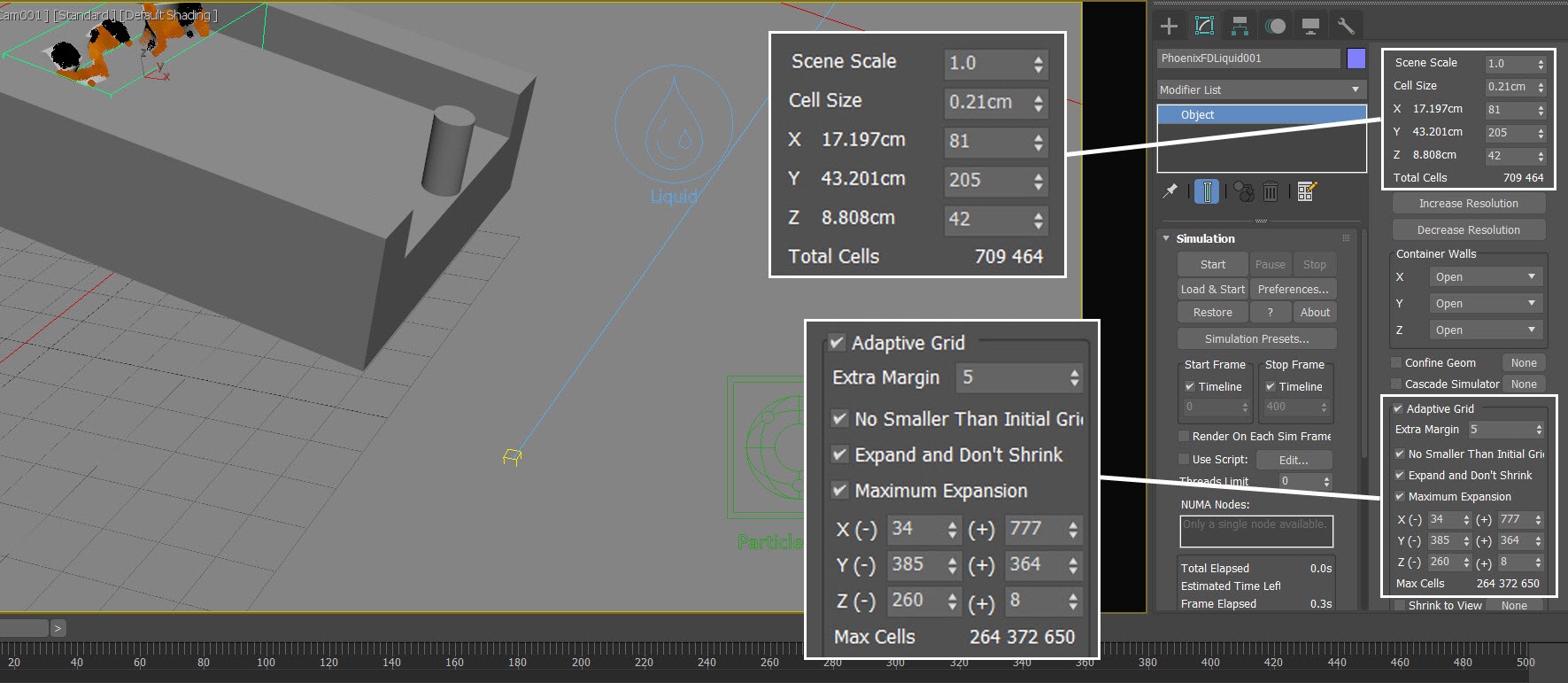
Select the Simulator and open the Grid rollout and set the following values:
Cell Size: 0.21 cm;
Size XYZ: [ 81, 205, 42 ];
Adaptive Grid: the Adaptive Grid algorithm allows the bounding box of the simulation to dynamically expand on-demand; Extra Margin to 5;
Enable Max Expansion: X: (34, 777), Y: (385, 364), Z: (260, 8) - to save memory and simulation time by limiting the Maximum Size of the simulation grid.
With the new Grid Resolution, new RGB Diffusion setting and the new mapped RGB in the LiquidSrc_Low_Viscosity Source, let's run the final simulation.
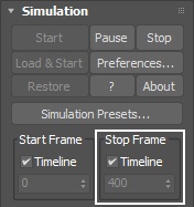
Go to the Simulation rollout → enable the Timeline option for the Stop Frame. Press the Start button to simulate.
Here is a preview animation up to this step.
Here is a Grid RGB preview animation.
Few steps back we used the Viscosity channel to preview the result, but the default color doesn't present the lava color well. Let's customize the Viscosity color swatch.
For the upper swatch, make it RGB (0, 0, 0); Give it value of 1.0.
For the lower swatch, make it RGB (255, 137, 0). Give it value of 0.001.

Here is a Grid Viscosity preview animation. The Viscosity channel presents the flowing lava better.
Phoenix allows you to preview the Viscosity and RGB channels at the same time.
To do that, go to the Preview rollout of the Simulator. Enable both Viscosity and RGB channels.

These pictures show the benefits of viewing Viscosity and RGB channels at the same time.
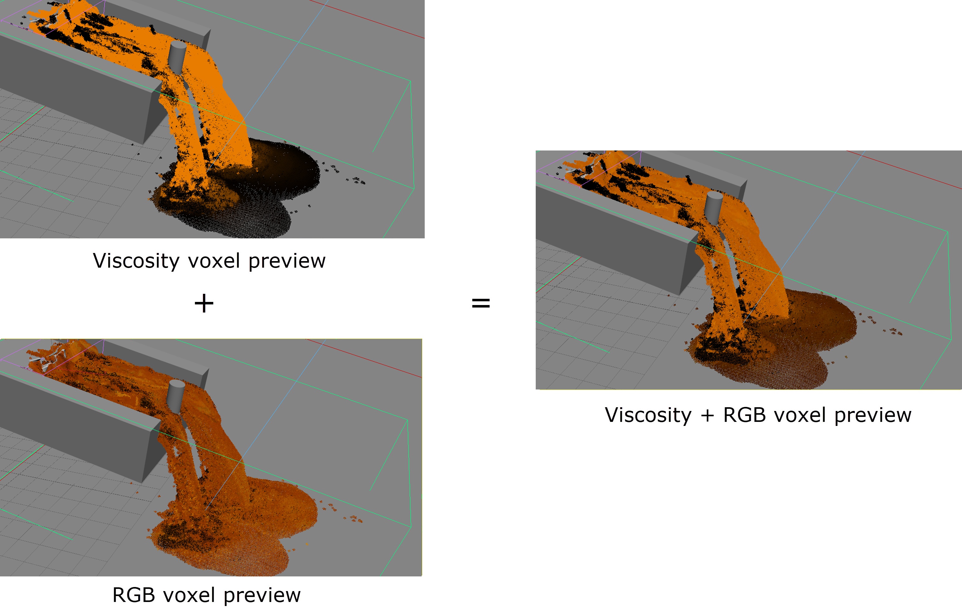
Now we have a much better visual representation of how the lava flow looks like and when it solidifies. We are ready to shade our lava flow.
Shading for the Lava Flow
The final material for the lava flow consists of 3 components:
- The Dark Lava material for the high viscosity part of the liquid;
- The Light Lava material for the low viscosity part of the liquid;
- The Mask that blends the two materials.
Let's create those three separately, and combine them using a V-Ray Blend Material.
Dark Lava Material
For the dark lava (the part with high viscosity), assign a V-Ray Material to the Simulator and name it Lava_dark. This material is the coat for the final Complex Lava material we create in the next section.
Set the Diffuse to RGB (35, 35, 36).
Set the Reflect to RGB (251, 251, 251).
Set the Reflection Glossiness to 0.56.

Here's a rendered image of the Lava with the Lava_dark material applied to the Simulator.
In this case, we choose to render the 415th frame, since it is representative. However, you can render out other frames as you like.

Light Lava Material
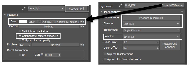
Create a VRayLightMtl and rename it to Light_lava. This material is the base for the final Complex Lava material we create in the next section.
Set the Color to RGB (0, 0, 0) - we use a Phoenix FD Grid Texture reading the simulation RGB Channel to drive the color of the emitted light.
Set the Color Multiplier to 25 - this affects the intensity of the emitted light.
Enable the Compensate camera exposure option.
Create a Phoenix FD Grid Texture and plug it into the Lava_light Light Material's Light Color input. Name it Grid_RGB.
Press the Pick a Phoenix Simulator button next to the Source Node parameter and select your Simulator from the popup menu. The name of the button should change according to the name of the simulator once you press the OK button.
Set the Channel to Grid RGB - this is the channel the texture reads from the cache files.
Set the Sampler to Spherical. You can think of the sampling process as Anti-Aliasing - the Box sampler gives you a rough texture, the Linear one smooths the colors and the Spherical produces the smoothest result.
Note that the Spherical sampling is 20-30% slower than Linear, so make sure to check if the additional sampling at the expense of render time is worth it with your setup.
When Compensate camera exposure is enabled, the intensity of the light material is adjusted to compensate the exposure correction from the physical camera.
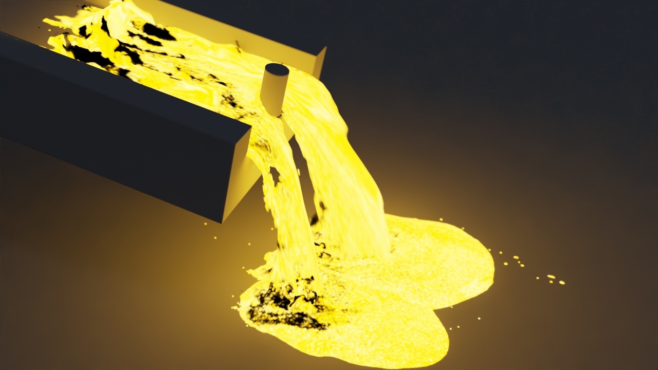
Here's a rendered image of the Lava with the Light_lava material applied to the Simulator.
The details from the RGB grid color are blown out because of the high Color Multiplier of the VRayLightMtl (Light_lava).
To rectify this, create a Color Correction node and connect it to the Grid_RGB (PhoenixFDTexmap). Rename the Color Correction node to color_correction_A.
Set the Color → Hue Shift to -20.0.
Set the Lightness → Brightness to 4.2.
Set the Lightness → Contrast to 12.0.
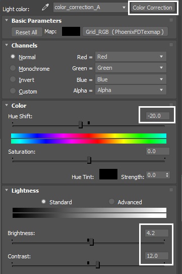
Here's a rendered image of the Lava with the Light_lava material applied to the Simulator. You can see better details coming from the color corrected Grid RGB.

Texture for the Mask
Now, let's create a Texture map for the Mask.
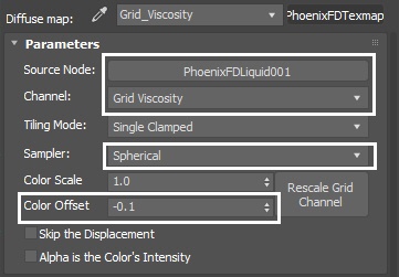
Create a Phoenix FD Grid Texture. Rename it to Grid_Viscosity.
Press the Pick a Phoenix Simulator button next to the Source Node parameter and select your Simulator from the popup menu. The name of the button should change according to the name of the simulator once you press the OK button.
Set the Channel to Grid Viscosity - this is the channel the texture reads from the cache files.
Set the Sampler to Spherical.
Set the Color Offset to -0.1.
Since the Mask is only a Texture map, let's temporarily create another V-Ray material (rename it Mask_Material), and put the Mask texture (Grid_Viscosity) in its diffuse slot, just to see how the texture map looks in the render.
Here's a rendered image of the Lava with the masked material applied to the Simulator. As you can see, all the details in the Grid Viscosity are revealed. However, in low contrast.
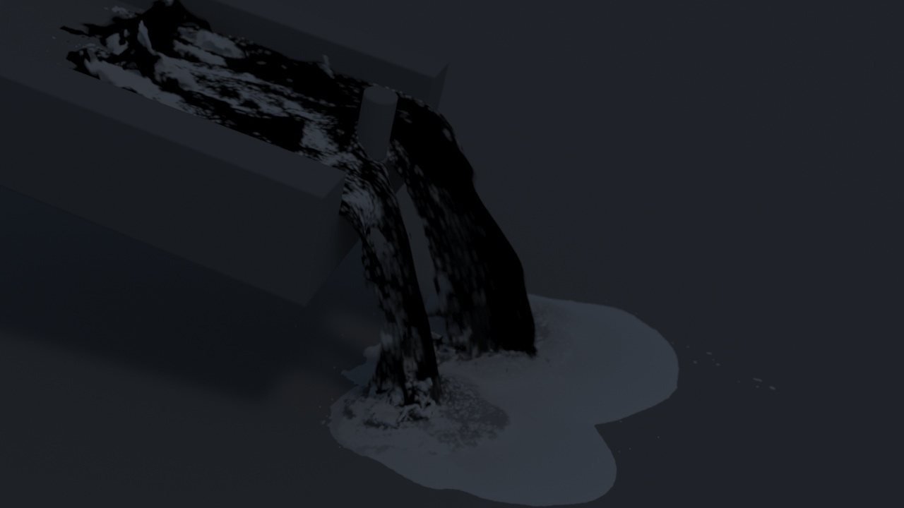
Let's tackle this next.
Create a Color Correction node to the Grid_Viscosity (PhoenixFDTexmap). Name the Color Correction node color_correct_B.
Set the Lightness → Contrast to 43.5.

Here's a rendered image of the Lava with the Mask_Material applied to the Simulator. Now the texture looks a bit more contrast, ready to act as a Mask.

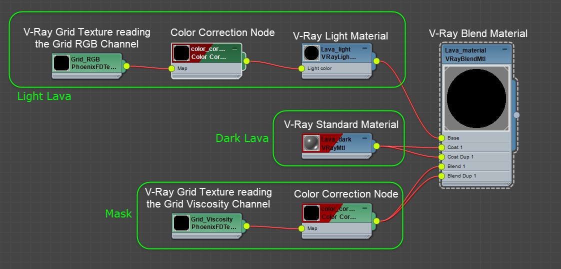
Complete the Lava Shader
The final material for the lava consists of the Dark_lava and Light_lava materials prepared in the previous sections.
A V-Ray Blend Material (renamed to Lava_material) is used at the final wrapper.
Plug the Light_lava to the Base of the V-Ray Blend Material.
Connect the Dark_lava to Coat 1.
Use the Mask texture for Blend 1.
See the attached picture.
Here's what we get from the render. In the next step, we will see how to improve this raw image with some post effects directly in the VFB.
V-Ray Frame Buffer
Open the V-Ray Frame Buffer and use the Create Layer icon to add layers for Lens Effects, Exposure, and Filmic tonemap.
Using V-Ray 5 as a render engine gives us the advantage of Filmic tonemap directly in the new VFB. However, if you are using an older version of V-Ray or 3ds Max 2017 or lower, you can get a similar effect by using a proper LUT.
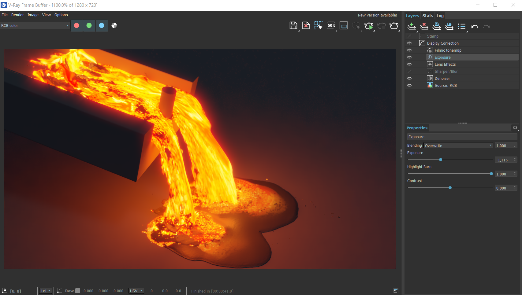
The final image is rendered using the V-Ray Frame Buffer with the color corrections and post effects set to:
Filmic tonemap:
Type - Hable;
Shoulder strength: 0.46;
Linear strength: 0.49;
Linear angle: 0.46;
Toe strength: 0.30;
White point: 10.36.
Exposure:
Exposure: -1.115;
Highlight Burn: 1.0;
Contrast: 0.0.
Lens Effects:
Size: 10.53;
Intensity:3.57;
Bloom: 0.4;
Threshold 1.0.
The Filmic tonemap allows you to simulate the film response to light within the VFB.
Feel free to use other values for the post effects depending on your preferences.

A V-Ray Denoiser is added to the final image. The Denoiser takes an existing render and applies a denoising operation to it after the image is completely rendered in order to remove the noise in the image.
This tutorial uses the Strong Preset.

And here is the final rendered result.